The following post was written in coordination with Dr. Thorsten Hans , Lear Corporation’s Comfort & Trim Simulation group leader. Dr. Hans completed his Engineering Diploma in mechanical engineering at the Technical University of Munich in 2012. He then acted as a research assistant in the carbon composites division of the Technical University of Munich, completing his doctorate in 2015. Subsequently, he worked as an FEA engineering consultant in the composites industry until 2019, whereupon he joined the Lear Corporation Engineering GmbH.

 

One of the main Transportation and Mobility (T&M) business drivers is the creation of novel customer experiences. No longer are customers just happy with traveling from point A to point B. They want to do so while experiencing a unique feeling in their vehicle. A major component of this is passenger thermal comfort. This well-being can be tuned through, for instance, the use of air conditioning or heating during hot or cold days, respectively. The most direct approach to satisfy passenger thermal comfort is to blow this cool or hot air through the interface between passenger body and vehicle seat, thereby creating a thermally regulated vehicle seat. In the past, design of temperature controlled vehicle seats, which includes the seat structure, foam layers, and fans, has taken place entirely on real-world thermal test benches. This approach is limiting though: one cannot access the full temperature or velocity field in the test domain. The current customer reference story aims to present a first-of-its-kind simulation workflow using a PowerFLOW–PowerTHERM coupled simulation to assess the thermal behavior of a vehicle seat provided by Lear Corporation. Lear Corporation is a global automotive supplier with sales of $20.9 billion in 2022 alone. It is the most vertically integrated seating supplier in the industry.

 

 

Climate seats themselves have fans integrated to generate an airflow through the cushion and/or backrest foam (see Figure 1). There are different cooling systems available: pressing/sucking environmental or actively cooled air through the seat, for example. Furthermore, to ensure the distribution of airflow through the seat, several material layers are assembled (see Figure 1). This is because, depending on the body region, different degrees of airflow are felt as “comfortable” (e.g. kidneys vs. buttock).

 

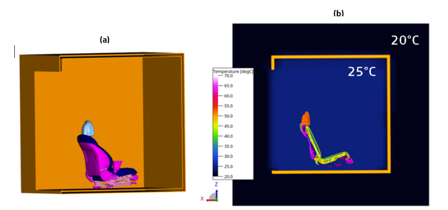
The real-world setup that is replicated in the digital domain consists of the following. The seat is positioned in a climate chamber with 25°C, while the air outside the chamber is set to an ambient value of 20°C (see Figure 2). In the real world, the seat is heated up by an infrared-lamp to 65°C surface temperature; in the simulation domain, this is merely imposed as a boundary condition on the seat surface’s leather layer. Subsequently, the lamp is switched off, the door of the climate chamber is opened and the air-conditioning of the seat is switched on. This represents when the simulation is initiated/started: the fans are turned on, blowing cool air through the seat layers.

 

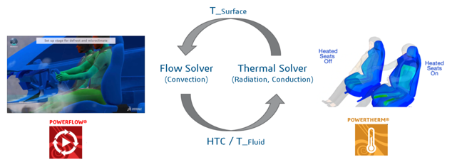
More now to the actual simulation workflow and modeling of components, such as fan and seat layers. The PowerFLOW-PowerTHERM coupling works as follows. PowerFLOW, the flow solver, models the convective effects of the surrounding air. Then, the heat transfer coefficients and wall-adjacent fluid temperatures are fed into the PowerTHERM solver. It computes, for the designated time interval, the radiation and conductive heat transfer mechanisms for the solid components in question. Subsequently, the solid surface temperatures are fed back into the convective PowerFLOW solver. This process repeats itself at predefined coupling intervals and is represented by Figure 3.

 

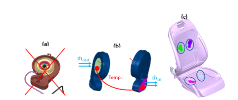
Moving on, the radial fans positioned in the seat foam were not explicitly simulated in order to save on simulation cost (see Figure 4a). Specifically, they were modeled using mass flow boundary conditions. To be able to obtain the correct airflow temperatures, a mapping from mass flow outlet (relative to the simulation domain) temperature to the mass flow inlet temperature was performed (see Figure 4b). A picture of the positioning of the fans in the seat can be seen in figure 4c. It is now apt to consider which components of the seat structure and foam should be considered as solid for conduction and fluid for convection. The plastic support, steel support and leather headrest were all modeled as solid shells (Figure 5a). Likewise, the solid foam and solid-like topper pad foam were also modeled as solids i.e., here too conduction was modeled as opposed to convection (Figure 5b). Meanwhile, the porous nature of the honey-comb spacers warranted their treatment as an adiabatic porous medium, which means this layer was modeled as a fluid with convection (Figure 5c). Finally, the leather layer too was considered as compact/dense, which means it was modeled as a solid volume for conduction. It is, however, important to note that 1mm radius perforations were added to the leather layer to allow for convective effects through this seat layer as well (Figure 5d).

 

Having discussed the setup of the digitized cooling heat seat scenario, temperature results are now looked at. This is done by looking at 3D temperature contour plots, 2D temperature contour plots, as well as 1D temperature evolution plots. First, the cushion (i.e. Kissen) is looked at. In Figure 6, the top row represents experimental data, while the bottom row displays simulation results. At a time of 0 seconds, both the experimental data and simulation data display a cushion with more or less a uniform temperature of 65°C – this is the temperature to which the seat was initialized.

 

 

 

 

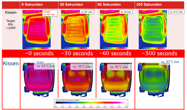
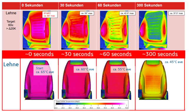
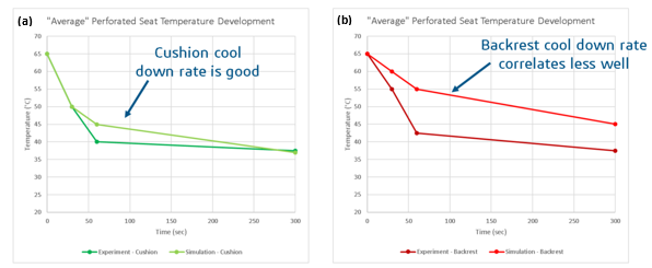
Meanwhile, at a time of 30 seconds, the experimental data shows a cushion temperature just below 50°C. This is only seen in the simulation data in the vicinity of the fans, suggesting that the conductive cooling through the leather layer is not as prominent in the digitized setup as it is in the real world. The trend continues as time progresses: at a time of 60 seconds after the chamber door is opened and the air-conditioning in the seat is turned on, the experimental data displays an almost uniform cushion temperature below 45°C, while in the simulation this is again only seen near the location of the fans. However, once the cool down has progressed to 300 seconds, a more comparative picture between experiment and simulation appears: both experiment and simulation show a cushion temperature of about 40°C. In Figure 8a, one can see a 1D evolution of the leather layer’s average temperature and one can clearly see that, during the temperature evolution, the simulation curve remains above the experimental curve until in the long-run both curves converge. Additionally, the cooling of the backrest (i.e. Lehne) is now analyzed. The corresponding 3D temperature contour plots are shown in Figure 7, where again the top row represents experimental data and the bottom row represents simulation data. Unfortunately, the comparison for the back rest is not as good as it is for the cushion. The cool down rate of the back rest is significantly slower in the simulation than it is in the experiment, suggesting elements in the back rest area are not cooled down as much as they should be in the simulation. This can be clearly seen in the 2D temperature field plots of Figure 9a-c. There, one can clearly see how the back rest area stays warm/hot, while the vicinity of the cushion cools down with time. By 300 seconds since cool down started, the average back rest temperature in the simulation still lies at about 45°C while in the experiment it lies at about 37.5°C. The 1D temperature evolution plot for the back rest, which can be seen in Figure 8b, shows that the simulation cool down curve is on average at least 8°C above the experimental data, particularly after a cool down time of 60 seconds.